Missing portion of honey bee genome: sequencing problem
Genome size variation can be vary high within a family, sometime even within a genus (e.g. monogonont rotifers, Caenorhabditis nematodes). However, within species genome size variation is unexpected (at least not without changes in ploidy).
Smith et al. 2019 sequenced three lineages of asexual cape honey bee after about twenty years of asexuality. The goal was to measure heterozygosity loss over this period of time in three independent replicates. The data were collected and reanalyzed for comparison with other asexual species in our recent preprint.
Observation
While two of the three samples shown a very honey-bee-like genome size (236 Mbp) and indeed the relatively high heterozygosity as reported by the original study (SRR8061554, SRR8061555, in Smith et al. 2019 denoted as sample A and sample C).
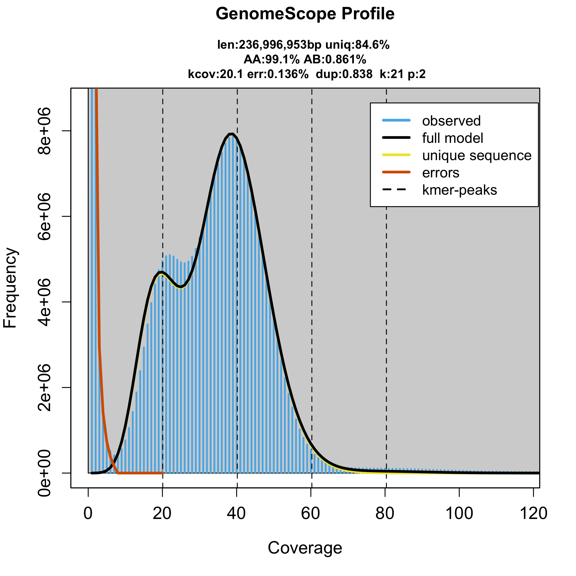
The third sample (SRR8061556; sample B), however, seems to have ~100 Mbp smaller genome size.
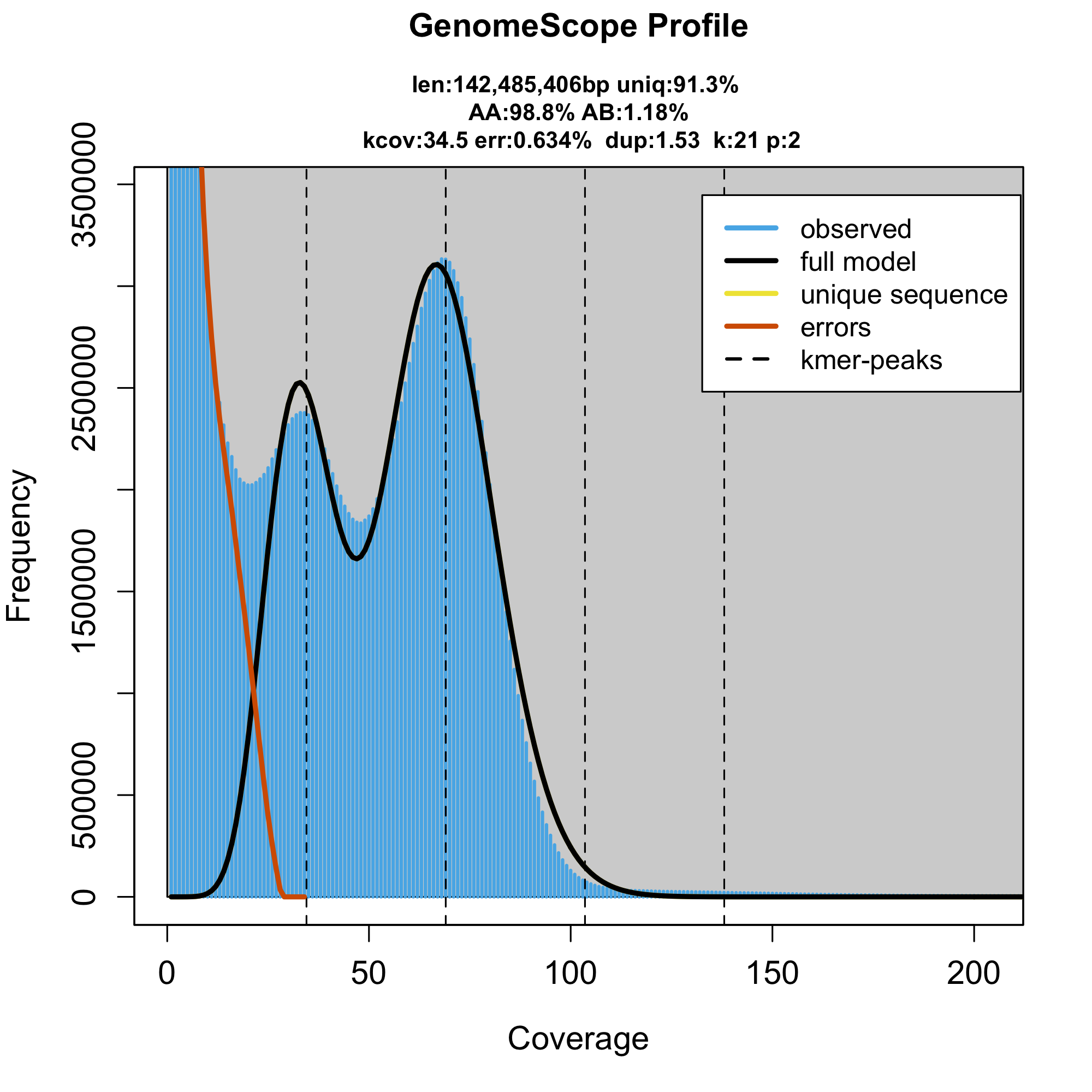
To make sure that it’s not a problem in the genome profiling software, we also did a back of an envelope calculation of the genome size using the total yield of the sequencing divided by the mean read depth reported in the paper. Such estimate will always overestimate the genome size as all the sequenced adapters, contaminations, mtDNA, etc. will inflate the estimate, but the calculation can serve as the maximal possible genome size estimate. The three samples have 12.2, 13.3 and 13.5 Gbp sequenced and their reported read depths are 46x, 50x and 69x respectively. The maximal genome size of the three samples is therefore 265, 266 and 195 Mbp. Again, the two samples are close to the expected genome size (236 Mbp), while the third sample is at least 41 Mbp smaller than the Apis melifera reference.
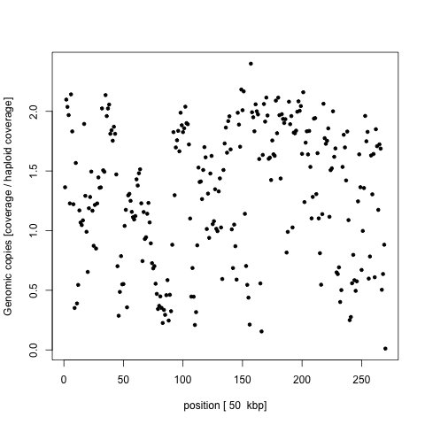
We wanted to figure out where are the missing bits of the genome and how comes that this is not reported in the original paper. We therefore mapped the sequencing library to the latest honey bee reference genome and calculated per 50k average depth along 16 chromosomes of the honey bee. For easier readability we again normalized per window depths by the expected haploid coverage. If the sequence is present in two copies in the genome (it’s a diploid genome), we expect the depth to be around 2 and the missing regions are expect to drop the coverage to 0. None of the chromosomes seems to be missing and moreover the coverage dropouts are scattered on all the chromosomes. As an example chromosome 11 shown on the following figure
a genome window could have non-integer normalized coverage only if it is partially present and partially absent in the genome, which would suggest micro deletions as the last possible biological explanation of the genome loss. If that is the case, we should be able to extract per base coverage depth and see that a large portion was not sequenced at all, while the rest have the 2n = 69x coverage. However, this is the histogram of the per base coverages with expectations marked by red line
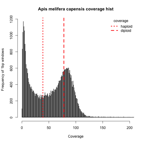
Only very few bases have really 0 coverage while the seems to be a strange coverage dropout on many locations in the genome without apparent explanation. It is very unlikely to find a biologically relevant explanation.
Explanation
It’s most likely an artifact of library prep. What exactly went wrong is hard to say, but my best guess is that there was not enough DNA after the library prep so they used a couple of rounds of PCR to amplify it and perhaps the bias could be related to very high AT-richness of the honey bee genome.
Methods
Used data:
- cape honey bee re-sequencing, SRA ids:
SRR8061556(the peculiar sample)SRR8061555(the alright sample),SRR8061554(also alright, but results not shown)
- honey bee reference genome Amel_4.5
Used software:
- KMC to generate kmer histogram
- GenomeScope for genome profiling
- bwa to map the reads to reference
- samtools depth analysis
- R plotting
Genome profiling
Taken from our recent preprint, but it is basically the very default genome profiling analysis.
# dl SRR8061556.sra file; convert it to fastq files; erase the .sra file
ls *.fastq > FILES
kmc -k21 -t16 -m64 -ci1 -cs10000 @FILES kmer_counts tmp
kmc_tools transform kmer_counts histogram kmer_k21.hist -cx10000
genomescope.R -i kmer_k21.hist -o output_dir -n apis_sample3
Remapping analysis
Let’s get the reference and reads
wget ftp://ftp.ensemblgenomes.org/pub/metazoa/release-45/fasta/apis_mellifera/dna/Apis_mellifera.Amel_4.5.dna.toplevel.fa.gz
map reads, filter low quality mapping (>20) and sort the reads.
bwa mem -M -t 30 -R "@RG\tID:1\tSM:Amel3\t\LB:Amel3" genome/Apis_mellifera.Amel_4.5.dna.toplevel.fa.gz reads/SRR8061556_{1,2}.fastq.gz | samtools view -h -q -20 | samtools sort -@10 -O bam - > Amel3_mapped.bam
First I need to extract chromosome sizes
samtools view -H data/Amel3_mapped.bam | grep "^@SQ" | cut -f 2,3 -d : | sed s/LN://g > data/Amel3_reference_sizes.tsv
Further I will extract every 5000th base to subsample the depth file to something plotable
samtools mpileup Amel3_mapped.bam -s | cut -f 7 > Amel3_per_nt.MQ
# extract mapping qualities
awk '{ if(NR % 5000 == 0){ print($0) } }' data/Amel3_per_nt.MQ > data/Amel3_per_nt_sample.MQ
# extract read depths
awk '{ if(NR % 5000 == 0){ print($0) } }' data/Amel3_per_nt.depth > data/Amel3_per_nt_sample.depth
testing if low coverage bases have a low mapping quality. The answer is no (plot not shown), the mapping qualities of lowly covered regions are about the same as the mapping qualities of normally covered regions.
library(gtools)
MQs <- read.table('data/Amel3_per_nt_sample.MQ', stringsAsFactors = F)$V1
depths <- as.vector(sapply(MQs, nchar))
mean_qualities <- as.vector(sapply(MQs, function(x){mean(asc(x))}))
mapping <- data.frame(depth = depths, MQ = mean_qualities)
mapping <- mapping[mapping$depth < 200,]

library(hexbin)
library(RColorBrewer)
rf <- colorRampPalette(rev(brewer.pal(11,'Spectral')))
r <- rf(32)
# Create hexbin object and plot
hexbinplot(MQ ~ depth, data = mapping, colramp=rf)
Looks like the low coverage bases are also well mapped. Suggesting that it’s not just mismapped reads that generate the low coverage pattern.